The Symmetries of the Quantum Kepler Problem (prime version)

This is a continuation of the discussion of the symmetries of the Kepler problem in the blog post Planets in the Fourth Dimension at the Azimuth blog. In this post we consider the quantum Kepler problem and investigate the Schrödinger equation. $ \newcommand{\rr}{\boldsymbol{r}} \newcommand{\pp}{\boldsymbol{p}} \newcommand{\xx}{\boldsymbol{x}} \newcommand{\vv}{\boldsymbol{v}} \newcommand{\uu}{\boldsymbol{u}} \newcommand{\ee}{\boldsymbol{e}} \renewcommand{\AA}{\boldsymbol{A}} \newcommand{\LL}{\boldsymbol{L}} \newcommand{\rrr}{\hat{\boldsymbol{r}}} \newcommand{\Ga}{\boldsymbol{\Gamma}} \newcommand{\ga}{\boldsymbol{\gamma}} \newcommand{\om}{\boldsymbol{\omega}} \newcommand{\al}{\boldsymbol{\alpha}} \renewcommand{\d}[1]{#1'} \newcommand{\dd}[1]{#1''} \newcommand{\ddd}[1]{#1'''} \newcommand{\dr}{\d{r}} \newcommand{\ddr}{\dd{r}} \newcommand{\drr}{\d{\rr}} \newcommand{\ddrr}{\dd{\rr}} \newcommand{\dddrr}{\ddd{\rr}} \newcommand{\dt}{\d{t}} \newcommand{\ddt}{\dd{t}} \newcommand{\dddt}{\ddd{t}} \newcommand{\dtau}{\d{\tau}} \newcommand{\ddtau}{\dd{\tau}} \newcommand{\dv}{\d{\vv}} \newcommand{\ddv}{\dd{\vv}} \newcommand{\dl}{\d{\lambda}} \newcommand{\du}{\d{u}} \newcommand{\dtheta}{\d{\theta}} \newcommand{\dphi}{\d{\phi}} $

Introduction

In the Kepler problem a particle with mass $m$ and position vector $\rr$ is moving under the influence of a central force $\boldsymbol{F}=-k \rr /r^3$, where $k$ is a constant that determines the strength of the force field and $r=|\rr|$ is the distance to the origin. Let $\ddot{\rr}$ be the second derivative of $\rr$ with respect to time. The equation of motion becomes \begin{equation} \label{motiontime} m\ddot{\rr} = -k\frac{\rr}{r^3}, \end{equation} We will consider the Kepler problem in the spacetime. We let a solution curve in spacetime be parameterised by a parameter $\lambda$ and let $\d{}$ mean differentiation with respect to $\lambda$. We have \begin{align} \drr &= \rr'_{\lambda}(\lambda)\\ \ddrr &= \rr''_{\lambda\lambda}(\lambda)\\ \dt &= t'_{\lambda}(\lambda)\\ \ddt &= t''_{\lambda\lambda}(\lambda). \end{align} The chain rule then gives that the equation of motion \eqref{motiontime} can expressed as \begin{equation} \label{motion} m\frac{\ddrr\dt-\drr\ddt}{\dt^3} = -k\frac{\rr}{r^3}, \end{equation}

Parameterisation with respect to time

We now choose not to define the parameterisation explicitly by some formulas \begin{align} \rr(\lambda)&=\text{ expression in $\lambda$}\\ t(\lambda)&=\text{ expression in $\lambda$} \end{align} but instead define the parameterisation implicitly by stating a constraint on $dt$. The simplest constraint is $dt=1$ and this corresponds to that the solution curve is parameterised with respect to time. Under this constraint the equation of motion becomes \begin{equation}\label{motiontimeparam} m\,\ddrr = -k\frac{\rr}{r^3}. \end{equation}

The standard Schrödinger equation

The time parameterised equation of motion \eqref{motiontimeparam} is the Euler equation of the variation problem \begin{gather} L(\rr,\drr) = \frac{m\drr^2}{2}+\frac{k}{r}\\ S = \int_\gamma Ld\lambda\\ \delta S=0, \end{gather} where $L(\rr)$ is the usual Lagrangian which is the difference between kinetic and potential energy. The action quantity $S$ can be made into an action function $S=S(t,\rr)$ by considering a central field of solution curves starting at a point $\rr_0$ at time $t_0$ and defining $S(t,\rr)$ to be the integral along such a solution curve to the point $\rr$ at time $t$. \begin{equation} S(t,\rr) = \int_{t_0,\rr_0}^{t,\rr} Ld\lambda \end{equation} The conjugate momentum of $\drr$ is $\pp=L_{\drr}=m\,\drr$ and the Legendre dual of the Lagrangian is the Hamiltonian. \begin{equation} H(\pp,\rr)=\pp\drr-L=\frac{\pp^2}{2m}-\frac{k}{r} \end{equation} The action integral can be rewritten as \begin{equation} S(t,\rr) = \int_{t_0,\rr_0}^{t,\rr} (\pp d\rr - Hdt) \end{equation} and the action function then has the differential \begin{equation} dS = \pp d\rr - Hdt \end{equation} We have that $S_{\rr}=\pp$ and $S_t=-H$, and we see that the action function fulfills the Hamilton-Jacobi differential equation \begin{equation} S_t = -H(S_{\rr},\rr) \end{equation} The Hamiltonian is conserved and is equal to an energy constant $E$ on the solution curves and the Hamilton-Jacobi equation then separates into two equations \begin{gather} H(S_{\rr},\rr) = E\\ S_t = -E \end{gather} and the total action function must separate into a spatial and a temporal part $S(t,\rr)=S(t)+S(\rr)$. The spatial equation is \begin{equation} H(S_{\rr},\rr) = E \end{equation} Instead of working directly with the action function $S(\rr)$ we express it as the logarithm of a dimensionless function $f(\rr)$ \begin{equation} S(\rr) = \hbar\log f(\rr), \end{equation} where $\hbar$ is the reduced Planck constant which has the dimension of action. We have that \begin{equation} S_{\rr}=\hbar\frac{f_{\rr}}{f} \end{equation} and the Hamilton-Jacobi differential equation can then be expressed as \begin{gather} H\left(\hbar\frac{f_{\rr}}{f},\rr\right) = E\\ \frac{\hbar^2}{2m}\left(\frac{f_{\rr}}{f}\right)^2-\frac{k}{r} = E\\ \frac{\hbar^2}{2m}f_{\rr}^2-\frac{k}{r}f^2=Ef^2\\ \frac{\hbar^2}{2m}f_{\rr}^2-\left(\frac{k}{r}+E\right)f^2=0.\label{HJ} \end{gather} We now allow $f$ to be complex-valued and not necessarily fulfill the equation \eqref{HJ}. Instead we integrate the left hand side over all of space and seek the function $f$ such that the variation of the integral is stationary. \begin{gather} K(f, f_{\rr}, \rr) = \frac{\hbar^2}{2m}f_{\rr}^2-\left(\frac{k}{r}+E\right)f^2\\ J = \int_{\mathbf{R}^3} K(f, f_{\rr}, \rr)dxdydz\\ \delta J = 0 \label{J} \end{gather} The Euler equation of the variation problem \eqref{J} is \begin{gather} \left(K_{f_{\rr}}\right)_{\rr} - K_f = 0 \\ \frac{\hbar^2}{m}f_{\rr\rr}+2(\frac{k}{r}+E)f = 0\\ -\frac{\hbar^2}{2m}f_{\rr\rr}-\frac{k}{r}f = Ef, \label{Sch} \end{gather} where $f_{\rr\rr}=f_{xx}+f_{yy}+f_{zz}$ is the Laplacian of $f$. Equation \eqref{Sch} is the time-independent Schrödinger equation.

Time dependence

The temporal Hamilton-Jacobi equation is \begin{equation} S_t = -E. \end{equation} We express the action function $S(t)$ as the logarithm of a dimensionless function $f(t)$ \begin{equation} S(t) = \hbar\log f(t). \end{equation} We have that \begin{equation} S_t = \hbar\frac{f_t}{f} \end{equation} The Hamilton-Jacobi equation then can be rewritten \begin{gather} \hbar\frac{f_t}{f} = -E\\ \hbar f_t = -Ef\label{HJt}\\ \hbar^2 f_t^2 = E^2f^2\\ \hbar^2 f_t^2 - E^2f^2=0\label{HJt2} \end{gather} We now allow $f$ to be complex-valued and not necessarily fulfill the equation \eqref{HJt}. Instead we integrate the left hand side of \eqref{HJt2} and calculate the function $f$ such that the variation of the integral is stationary. \begin{gather} K(f,f_t,t) = \hbar^2f_t^2 - E^2f^2\\ J = \int_{\mathbf{R}}K(f,f_t,t)dt\\ \delta J = 0\label{JJJJ} \end{gather} The Euler equation of the variation problem \eqref{JJJJ} is \begin{gather} \left(K_{f_t}\right)_t - K_f = 0 \\ \hbar^2f_{tt}+E^2f=0\\ \hbar^2f_{tt}=-E^2f\\ \hbar f_t = -iEf\\ i\hbar f_t = Ef \end{gather} where the next-to-last step is "taking the square root" to reverse the squaring of \eqref{HJt} and choosing the sign correspondingly.

The adapted parameterisation

We return to the parameterisation independent equation of motion \eqref{motion}. We take the scalar product with $\drr/\dt$ on both sides and integrate to get \begin{gather} m\frac{\ddrr\dt-\drr \ddt}{\dt^3} \cdot \frac{\drr}{\dt} = -k\frac{\rr}{r^3} \cdot \frac{\drr}{\dt} \\ \frac{m}{2}\left|\frac{\drr}{\dt}\right|^2 - \frac{k}{r} = E, \end{gather} where the integration constant $E$ is the total energy of the system. We assume that the energy is negative, $E<0$, and we can then define a characteristic speed $V=\sqrt{-2E/m}$, a characteristic radius $R=-k/(2E)$ and a characteristic time $T=R/V=-k\sqrt{-m/(8E^3)}$. We now state a new different constraint $\dt=r/V$, which specifies the parameterisation indirectly. In the equation of motion \eqref{motiontime} we substitute $r=V\dt$ and get \begin{gather} mV^2\frac{r\ddrr-\dr\drr}{r^3} = -k\frac{\rr}{r^3} \\ \ddrr = -\frac{R\rr}{r} + \frac{\dr\ddrr}{r}. \end{gather} The radial component of $\ddrr$ is $\ddr-(|\drr|^2-(\dr)^2)/r$ and the radial equation of motion becomes \begin{align} \ddr-\frac{|\drr|^2-\dr^2}{r}&=-R+\frac{\dr^2}{r}\\ \ddr&=\frac{|\drr|^2}{r}-R\\ &=\frac{R^2-(R-r)^2}{r}-R \\ &=-(r-R), \end{align} which is equivalent to \begin{equation} \dddt=-(\dt-T). \end{equation} By differentiating the equation of motion and using the result for the radial equation of motion we further get that \begin{equation} \dddrr=-\drr. \end{equation}

Symmetry group

Let $\vv = (\dt-T)\ee_t+\drr$ be a vector denoting the 4-velocity relative to the characteristic 4-velocity $T\ee_t$. The energy equation and the equations of motion can then be expressed as \[ \begin{cases}||\vv||=R\\ \ddv=-\vv\end{cases} \] These equations are invariant under the symmetry group $O(4)$ and we see that the $\vv$-vector will trace a great circle on the sphere $||\vv||=R$ with constant speed $||\dv||=R$. We also see that the great circles are parameterised by their angle and that the parameter $\lambda$ is the angle of the circle.

Conserved spacetime bivector

Since $\vv$-curves are great circles with constant speed we have that $\Ga=\vv\wedge \dv$ is a conserved spacetime bivector. It can be computed as \begin{align} \Ga&=\vv\wedge \dv\\ &=T\ee_t\wedge\frac{1}{T}((\dt-T)\ddrr-\ddt\drr)+\drr\wedge \ddrr\\ &=T\ee_t\wedge-\frac{1}{\dt}((\dt-T)\rr+\ddt\drr)+\frac{T}{\dt}\rr\wedge \drr\\ &=T\ee_t\wedge-\frac{1}{r}((r-R)\rr+\dr\drr)+\frac{R}{r}\rr\wedge \drr. \end{align} The bivector consists of a conserved spatal bivector $\LL=\frac{R}{r}\rr\wedge \drr$ and a conserved space vector $\AA=\frac{1}{r}((r-R)\rr+\dr\drr)$. The great circles are projected onto the spatial subspace as centered ellipses. Such an ellipse lies in the plane given by the bivector $\LL$ and has major semiaxis $R$ and area $\pi|\LL|$.

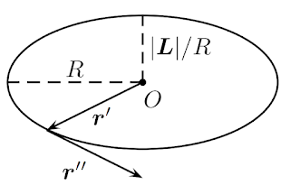To see the meaning of $\AA$ we observe that when $\drr$ points at a covertex of the ellipse we have that $\AA=(r-R)\ddrr/R$ and hence is directed along the major axis. Its length is then $|\AA|=r-R=V|\dt-T|=\sqrt{R^2-(|\LL|/R)^2}$ since $V|\dt-T|$ is the height from the covertex to the corresponding point on the great circle. This length relationship is one of the defining properties of a focus of an ellipse and we conclude that $\AA$ points to one of the focuses of the ellipse.

With the help of the vector $\AA$ the equation of motion for $\ddrr$ can be expressed as: \[ \ddrr=-(\rr-\AA) \] Also the $\ddrr$-vector describe the same ellipse as the $\drr$-vector and hence we conclude that the orbits for negative energies of the Kepler problem are ellipses with the origin as one of the focuses.

The conserved bivector $\LL$ can be identified with the angular momentum bivector \[ \LL_{\textrm{am}} = \rr\wedge m\frac{d\rr}{dt} = \rr\wedge m\frac{\drr}{\dt} = \frac{m}{T}\LL \] and the the conserved vector $\AA$ that gives the displacement of the force center corresponds to the Laplace-Runge-Lenz vector which in three dimensions is defined as \[ \AA_\mathrm{LRL}=-m\frac{d\rr}{dt}\times\LL_{\textrm{am}}-mk\frac{\rr}{r}. \] In $n$ dimensions the cross product generalises to the geometric product and we get that \[ \AA_\mathrm{LRL}=-m\frac{d\rr}{dt}\LL_{\textrm{am}}-mk\frac{\rr}{r}=\frac{m^2}{V^2}\AA. \]

The adapted Schrödinger equation

We have that the spacetime velocity $\uu=\dt\ee_t+\drr$ can be decomposed as \begin{equation} \uu = T\ee_t + (\dt-T)\ee_t+\drr \end{equation} The first component $T\ee_t$ is a constant velocity in time and the second component $(\dt-T)\ee_t+\drr$ is a velocity of constant speed $R$ along a circle $V^2(t-T\lambda)^2+(\rr-\AA)^2=R^2$. A solution curve in spacetime is a helix-like curve on an elliptic cylinder. The base is the ellipse of the spatial orbit with center at $\AA$ and the axis of the cylinder is along the time direction. On this cylinder we put coordinates $\theta$ and $\phi$ such that the the coordinate curves of $\theta$ are are tilted circles and the coordinate curves of $\phi$ are longitudinal lines on the cylinder. That is, from a circular cylinder with longitudinal coordinate $\theta$ and angular coordinate $\phi$, apply a shearing transformation that takes the cylinder into an elliptic cylinder. The coordinate circles of constant $\theta$ will then be tilted circles on the elliptic cylinder. The coordinate $\phi$ is taken to be an ordinary angular coordinate of the circle such that $2\pi$ is a whole turn and $R\phi$ is the length of the circular arc. The coordinate $\theta$ is a corresponding dimensionless longitudinal coordinate such that $T\theta$ is the elapsed time on the line segment. It is in these coordinates that the spacetime velocity separates \begin{equation} \uu = \underbrace{T\ee_t}_{\text{along $\theta$}} + \underbrace{(\dt-T)\ee_t+\drr}_{\text{along $\phi$}} \end{equation} and we have that \begin{gather} \dtheta = 1\\ \dphi = 1. \end{gather} The action of $\phi$ is $2\pi$ times the angular momentum associated with $\phi$. The angular momentum is $mVR=2ET=-k\sqrt{-m/(2E)}$. Also the $\theta$-angle has an associated action of equal amount $2\pi mVR$. The action function is \begin{equation} S(\theta,\phi) = \int_{\theta_0,\phi_0}^{\theta,\phi}\left(2ETd\theta+2ETd\phi\right) \end{equation} The differential of the action function is \begin{equation} dS = 2ETd\theta + 2ETd\phi \end{equation} and we have that \begin{gather} S_{\theta} = 2ET\\ S_{\phi} = 2ET \end{gather} We express the action as the logarithm of a dimensionless function $f(\theta,\phi)$ \begin{equation} S(\theta,\phi) = \hbar\log f(\theta,\phi) \end{equation} and we have that \begin{gather} S_{\theta} = \hbar\frac{f_\theta}{f} = 2ET\\ S_{\phi} = \hbar\frac{f_\phi}{f} = 2ET \end{gather} We continue for the moment with the equation for $\phi$. It can be rewritten as \begin{gather} \hbar\frac{f_\phi}{f} = 2ET\\ \hbar f_{\phi} = 2ETf \label{A2} \\ \hbar^2f_{\phi}^2 = 4E^2T^2f^2\\ \hbar^2f_{\phi}^2 - 4E^2T^2f^2 = 0 \label{A1} \end{gather} We now allow $f$ to be complex-valued and not necessarily fulfill the equation \eqref{A1}. Instead we integrate the left hand side and seek the function $f$ such that the variation of the integral is stationary. \begin{gather} K(f, f_{\phi}, \phi) = \hbar^2f_{\phi}^2 - 4E^2T^2f^2\\ J = \int_0^{2\pi} K(f, f_{\phi}, \phi)d\phi\\ \delta J = 0 \label{JJJ} \end{gather} The Euler equation of the variation problem \eqref{JJJ} is \begin{gather} \left(K_{f_{\phi}}\right)_{\phi} - K_f = 0 \\ \hbar^2f_{\phi\phi}+4E^2T^2f=0\\ \hbar^2f_{\phi\phi}=-4E^2T^2f\\ \hbar f_{\phi} = i2ETf \label{Sch3} \end{gather} where the next-to-last step is "taking the square root" to reverse the squaring of \eqref{A2} and choosing the sign correspondingly. The equation \eqref{Sch3} is the adapted Schrödinger equation. It has the solution \begin{gather} f(\phi) = Ce^{i\alpha\phi},\\ \alpha=\frac{2ET}{\hbar}=\frac{k}{\hbar}\sqrt{-\frac{m}{2E}}\\ C\text{ is a complex constant} \end{gather} The quantity $\alpha$ must equal a positive integer $n=1,2,3,\dots$ and we get \begin{gather} \frac{k}{\hbar}\sqrt{-\frac{m}{2E}} = n\\ E = -\frac{mk^2}{2\hbar^2n^2} \end{gather} In a hydrogen atom the force constant $k$ is $k=e^2/(4\pi\epsilon_0)$, where $e$ is the elementary charge and $\epsilon_0$ is the vacuum permittivity. We have \begin{equation} E = -\frac{me^4}{2(4\pi\epsilon_0)^2\hbar^2n^2}. \end{equation} For the $\phi$-coordinate, we have the same equation and the total solution is \begin{gather} f(\theta, \phi) = f(\theta)f(\phi)= C_1e^{i\alpha\theta} C_2e^{i\alpha\phi} = Ce^{i\alpha(\theta+\phi)},\\ \alpha=\frac{k}{\hbar}\sqrt{-\frac{m}{2E}}=\text{ positive integer}\\ C_1,C_2,C\text{ are complex constants} \end{gather}

Spin-1/2

The solution to the adapted Schrödinger equation is a complex exponential which spatial part is defined on an ellipse. This ellipse is the orbit of the corresponding classical Kepler problem. The complex exponential can be physically interpreted as a one-dimensional travelling wave, for example a travelling longitudinal wave around the ellipse. The amplitude and phase of the wave is collected in the complex amplitude $C$ of the complex exponential. If we were to instead interpret the wave as a travelling transverse wave, we would have a two-dimensional wave that would allow for two polarisation modes. Each of the polarisation modes would have an amplitude and a phase which can be collected in two complex amplitudes $C_{+}$ and $C_{-}$. These constitute a complex two-dimensional vector and $SU(2)$ has its natural action on this vector. The travelling transverse wave realises a spin-1/2 system.